Data Acquisition

Data acquisition often serves as the foundational step in test programs, tasked with collecting data that represents physical quantities or signals from hardware devices.

Utilizing Device Drivers

No matter what data acquisition device is being used, having a device-specific driver designed for LabVIEW can drastically reduce the complexity of programming. Hardware devices used for data collection are diverse, ranging from various card-based devices, traditional instruments, to embedded smart devices. While their drivers may differ, their functionalities and usage methods are generally similar: they involve sequentially opening or initializing the device through the driver's interface VIs, configuring the device as needed, reading data from the device, and ultimately closing the device.

NI-produced hardware devices typically come equipped with LabVIEW drivers. Many devices from other manufacturers also include LabVIEW drivers; users can obtain these drivers by contacting the respective hardware manufacturers.

For widely used instruments, LabVIEW provides a "Find Instrument Drivers" tool to help locate and install their drivers. This tool can be found under the menu path: "Tools -> Instruments -> Find Instrument Drivers".

The image below is the launch interface of the "Find Instrument Drivers" tool.

To use this tool, you must first register for and log into an ni.com account. You can then search for the drivers of specific instruments using the manufacturer name and keywords. The following image shows the results of such a search.

Utilizing C Language Drivers for Hardware Devices

Some hardware devices may lack LabVIEW drivers but often provide C language drivers instead. These drivers are typically delivered in the form of DLLs, which include the necessary functions for controlling hardware devices or reading data. Additionally, a .h header file is provided to declare the definitions of these functions.

In LabVIEW, these types of drivers can be used directly by employing Call Library Function (CLN) nodes to invoke the driver functions within applications. However, using CLN nodes isn't the most straightforward approach. A better strategy involves wrapping the C language drivers into a form compatible with LabVIEW before utilizing them in LabVIEW.

A straightforward wrapping method involves using LabVIEW's "Import Shared Library" tool to import all functions from the DLL into LabVIEW as VIs. Utilizing driver functionalities provided as VIs in test programs is significantly more convenient than using CLN nodes directly. This is because VIs can include extensive information, such as explanations of the functions, range of parameters, and more.

If a driver is frequently used, it merits the effort to design it to be both professional and user-friendly. Redesigning the driver structure allows for a departure from merely wrapping each DLL function into a VI; instead, each VI's functionality can be designed in the most intuitive manner for LabVIEW use. A VI may call multiple DLL functions, offering enhanced functionality. Such drivers can be inspired by IVI instrument drivers used in LabVIEW, which are also created by wrapping DLLs.

Developing Drivers

Some infrequently used or simpler data acquisition devices may not provide any form of drivers, instead being controlled through commands represented as strings or numerical values sent from the program to the instruments.

Instruments typically connect to computers through GPIB, USB, ethernet, or other types of data cables. To send data to these devices in LabVIEW, the "Instrument I/O -> VISA" functions are utilized, with VISA Write and VISA Read being the most frequently used.

By specifying the "VISA resource name" parameter in the correct format, data can be transmitted to a device connected through a specific type of data cable. Detailed instructions on this resource name's format are provided in LabVIEW's help documentation.

Direct use of VISA functions in applications, akin to direct use of CLN nodes, is less than ideal due to its lack of intuitiveness and cumbersome configuration. Therefore, for hardware devices without existing drivers, it's viable to develop your own drivers for application use. Essentially, a driver consists of a collection of VIs, each incorporating the device's most commonly utilized functionalities. An instrument's typical functions are often composed of one or several commands. For example, to read a measurement value from an instrument, a command to perform the measurement must first be sent, followed by a command for the instrument to send data, and then reading the data. Accordingly, a driver VI is made up of one or more VISA functions. Below is a VI from the LabVIEW-built Agilent 34401 multimeter driver, with its functionality primarily executed through VISA functions to send commands to the instrument.

When creating a driver, the initial step is to design its structure. This includes deciding which VIs the driver should contain, the functionality of each VI, and their implementation. Driver design should take inspiration from existing drivers or standards, as adopting a pre-designed interface saves considerable time and effort. Users of the driver will also benefit from its familiarity with other drivers, thereby reducing the learning curve.

Interchangeable Virtual Instrument Drivers

The Interchangeable Virtual Instrument (IVI) driver standards, developed by the Interchangeable Virtual Instrument Foundation, are designed to enable instrument interchangeability during runtime in test programs.

Typically, standard drivers create a dependency between the test software and specific hardware devices and drivers. If a test program is moved to a computer lacking the necessary drivers, it won't operate. Furthermore, if a different instrument is connected to another computer, the test program must be rewritten to incorporate the new instrument's driver. The distinction of IVI instrument drivers lies in their ability to switch to different instrument models without necessitating a rewrite or recompilation of the test program, thereby allowing the use of various models for testing purposes.

For interchangeability, the IVI Foundation extracted common features across similar instruments and set standards for each type, such as oscilloscopes, digital multimeters, spectrum analyzers, etc. Each instrument category has its "Class Driver" (IVI Class Driver), which encompasses common properties and functions. Runtime control of the instruments is achieved by the class driver calling specific functions from each instrument's individual specific driver (IVI Specific Driver). For instance, IviDmm serves as the class driver for digital multimeters, with fl45 being the specific driver tailored for the Fluke 45 multimeter model.

Multiple specific drivers for different models of the same instrument type might be installed on a computer. The IVI configuration file specifies which specific driver should be utilized by the class driver. Installing LabVIEW also installs the "Measurement & Automation" (MAX) software, an NI proprietary application for hardware device configuration, facilitating intuitive adjustments in the IVI configuration file settings.

Instrument interchangeability in test programs is made possible by calling the class driver, which references the IVI configuration file to select the appropriate specific driver. If instruments within the system are replaced, merely adjusting the IVI configuration file suffices without any need for application modification, thus ensuring the test system's versatility.

IVI drivers, compared to traditional instrument drivers, are better suited for sophisticated applications and developing extensive testing systems. For instance, I developed a calibration program set intended for use across various calibration labs, each equipped with different instruments. Writing individual programs for each lab would be inefficient. Utilizing the IVI architecture for these calibration programs proved to be an optimal solution. With a single software version and each lab configuring their instruments within MAX, the calibration software could be universally applied.

Software Timing

In LabVIEW programs, it's common to encounter scenarios where certain code needs to be executed at timed intervals. Depending on the application, the required precision for these intervals can vary significantly. Some programs might have relatively lax timing requirements. For example, consider the following program:

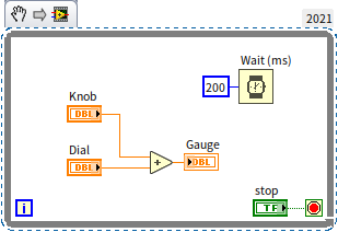
This program is set to perform calculations and update the interface every 200 milliseconds. The precision required for its timing is quite low; even a 50% deviation from the 200-millisecond target would not significantly impact the program's functionality.

Conversely, other programs demand much higher timing precision. When acquiring signals using data acquisition devices, for instance, the precision requirements could be thousands of times more stringent than those of the previously mentioned program. In the realm of high-speed data acquisition, timing errors must be minimized to the order of 10^-9^ seconds.

Timing Functions and VIs

LabVIEW offers several ways to implement timing functions, with the simplest being the use of provided timing functions and VIs. Commonly used timing-related functions or VIs include "Tick Count", "Wait", "Wait Until Next ms Multiple", "Time Delay", and "Elapsed Time", all located in the "Programming -> Timing" function palette.

The program illustrated below utilizes two "Tick Count" VIs to calculate the duration required for executing a code segment. To implement timing, it continuously checks the current time, executing the task again once the interval since the last execution reaches a specified duration, thereby fulfilling the timing requirement.

The "Elapsed Time" VI functions similarly to "Tick Count", albeit with additional features.

For simpler timing requirements, direct usage of the "Wait", "Wait Until Next ms Multiple", or "Time Delay" functions suffices, all of which are fundamentally identical in operation. They all discern a minimum wait or delay time of 2 milliseconds, with their main distinction lying in precision. "Wait" and "Time Delay" share similar precision levels, each potentially deviating by several milliseconds upon execution. "Wait Until Next ms Multiple" is noted for its higher precision.

Thus, for programs where precision requirements are modest, such as those needing only to refresh a display every 200 milliseconds, either "Wait" or "Time Delay" is appropriate. For data acquisition programs with moderate precision requirements, "Wait Until Next ms Multiple" might be an option. Should higher precision be necessitated, additional timing methodologies should be considered.

In LabVIEW programs, when timing functionalities are needed, the most common approach involves using the "Wait" and "Wait Until Next ms Multiple" functions in conjunction with loops. Therefore, this discussion will primarily focus on comparing these two functions.

• The "Wait" function is relatively straightforward: it takes an input parameter of n milliseconds, and each time the program encounters this function, it pauses for n milliseconds before continuing with the subsequent code execution.
• The "Wait Until Next ms Multiple" function is a bit more complex: given an input parameter of n milliseconds, each time the program reaches this function, it pauses. The function wakes up every n milliseconds, and upon awakening, it resumes the subsequent code execution.

Generally, if a program doesn't require very precise timing, the choice between "Wait" and "Wait Until Next ms Multiple" doesn't significantly matter, and either function can be used. Only in situations where high precision in timing is necessary should their subtle differences be considered.

Explaining these concepts in the abstract can be challenging, so let's look at a program example. Suppose in the depicted program, both "Read Data" and "Write Data" functions run for n milliseconds (this runtime applies to these sub-programs in other examples within this section as well). If n is less than 50, typically, each loop iteration in the two programs takes about 100 milliseconds.

Precision

However, there's a difference in timing precision between the two programs. The precision of using "Wait Until Next ms Multiple" within a loop far surpasses that of using "Wait".

In non-real-time operating systems like Windows, the accuracy of timing functions is relatively low, and experiencing a few milliseconds of deviation per execution is normal.

With the "Wait" function, timing starts anew each time the loop encounters it, leading to the accumulation of errors. For example, if there's an error of four or five milliseconds per iteration, the total error could reach fifteen milliseconds or more after five iterations.

On the other hand, the "Wait Until Next ms Multiple" function doesn't calculate delay at each invocation. Assuming the function starts timing from zero, it predetermines its wake times right from the program's start: at 100ms, 200ms, 300ms, and so on. If there's an error of ±4 milliseconds, then its actual wake times could be 100±4ms, 200±4ms, 300±4ms, etc., without such errors accumulating.

Timing the First Iteration

Let's examine the runtime differences when using the "Wait" and "Wait Until Next ms Multiple" functions. What are the values of x-y after running the programs below, assuming we ignore any errors?

In the program utilizing the "Wait" function, each delay adds 500 to x-y; after five 100 millisecond delays, the sum is 500 milliseconds.

In contrast, the program employing the "Wait Until Next ms Multiple" function offers an x-y value that is uncertain but will range between 400+2n and 500. This variance occurs because the "Wait Until Next ms Multiple" function doesn’t anchor its timing to the program's start time. Although it guarantees a wake-up interval of 100ms, the exact moment of the first wake-up varies, potentially occurring at any point within the first 0 to 100ms.

If precise timing of 100 milliseconds for the loop's first iteration is necessary, the solution is straightforward: use the "Wait Until Next ms Multiple" function for an initial sleep phase without action, then commence its operational use from the second iteration onwards. As depicted below, this approach consistently yields a result of 500 for x-y with every program run.

Parallel vs. Serial Execution

The programs discussed previously have the delay function and other code operating in parallel. This setup allows the loop iteration time to be primarily dictated by the delay function's input parameter, assuming the remaining code executes in negligible time. Sometimes, however, the delay function must operate serially, especially if a specific delay between two points is required.

Serial configuration significantly impacts the accuracy of the "Wait" function. For instance, the left-hand program now requires a total of 2n+100 per loop iteration. The variable n, influenced by the computer's performance and CPU load, introduces substantial timing variability.

Conversely, the "Wait Until Next ms Multiple" function's operational effectiveness remains unchanged in both parallel and serial configurations (when 2n<100), as it focuses solely on maintaining consistent wake-up intervals.

Utilizing Event Structures

Event structures come with a timeout event branch. By supplying a positive integer, like "25", to the structure's timeout input, LabVIEW automatically triggers the code within the timeout event branch every 25 milliseconds.

Employing the event structure's timeout event for timing offers precision akin to the "Wait" function. If the program already includes an event structure and necessitates timing functionality, integrating timing into the existing event structure is a practical first step.

For instance, if the application involves displaying an animation sequence that requires refreshing every 30 milliseconds and the program utilizes an event structure for interface management, the animation refresh code can be conveniently inserted into the timeout handling branch of the event structure:

Timing Loops

The common drawback of the timing methods we've previously discussed is their relatively low precision. For high-precision timing, reliance on specialized hardware devices is often required.

Most data acquisition devices come equipped with their own hardware timing features. Thus, when using these devices, it's typically the device's internal timer, not the software, that controls the interval between each sample.

However, when software needs to manage timing with high precision, especially on embedded devices, timing loop structures can be employed. These structures offer significantly higher precision than the methods previously discussed. In a test program I once worked on, relying on the "Wait" function for timing led to several minutes of error after an hour of operation. Switching to the "Wait Until Next ms Multiple" function reduced the error to under a minute. Ultimately, utilizing a timing structure brought the error down to just a few seconds.

Additionally, for programs running on PCs, timing loops should be considered when precise timing is required, multiple timing levels need to be set, or there's a need to dynamically adjust timing functions.

Timing loops are found in the "Programming -> Structures -> Timing Structure" function sub-palette. This sub-palette includes "Timed Loop", "Timed Sequence", among other nodes. Their functions and usage are relatively straightforward, and readers are encouraged to refer to the "Help File" for more information, hence this book will not delve into them in detail.

Hardware Timing

Setting the sampling rate is crucial when using data acquisition devices. For example, if a program needs to read 100 data points per second, equating to a 10-millisecond interval between samples, you might think of employing LabVIEW's delay functions. Placing a loop with a 10-millisecond delay within it to read a data point with each iteration seems logical.

This approach, however, has several issues: first, on computers running non-real-time operating systems like Windows, delay functions can support a minimum of only 1 millisecond, making intervals below 1 millisecond unachievable using this method. Second, the precision of delay-based methods is relatively low. For instance, setting a delay for 1 millisecond could result in errors several times larger than the intended delay, which is unacceptable for most data acquisition applications requiring high precision. Furthermore, reading from the data acquisition device after every single data point in high-volume data scenarios is inefficient.

In fact, most data acquisition devices are equipped with high-precision internal clocks. Therefore, it's preferable to utilize the hardware's clock for setting the sampling interval, rather than software-based timing methods. The hardware's driver software includes settings for the sampling interval (sometimes referred to as "sampling rate"), enabling efficient data reading by batching several data points together.

Continuing with the audio capture example, if a program needs to continuously capture and display audio signals, using Express VI would be unsuitable. The Sound Capture Express VI is intended for single, fixed-length audio captures. For continuous capture, VIs from "Programming -> Sound -> Input" serve as the sound card's driver program VIs.

Below is a diagram illustrating a simple program for capturing audio signals. Initially, the "Configure Sound Input" VI is used to set the sampling rate to 22050, configuring the sound card's clock accordingly. With a set number of 5000 samples, the sound card's hardware collects 5000 data points before transferring them to memory in one go. The program then visualizes these data points. Displaying 5000 data points at once is much more efficient than displaying one data point at a time over 5000 iterations.