Case and Sequence Structures

Case Structure

In LabVIEW, a Case Structure consists of several branches. Each branch contains its unique set of subdiagram. The structure operates by examining the input condition and executing the code in only one of its branches, depending on this condition. This is akin to the if else and switch statements in C language.

The image above illustrates a Case Structure, which shares a resemblance to the Loop Structure we previously discussed. It's enclosed within a rectangular frame, but distinctively, it houses multiple branch pages. Notably, only one page's content is visible at any given moment.

On the Case Structure's left, a small rectangle marked with a question mark serves as the case selector. The structure determines which branch to execute based on the data received by this selector. Above the structure, there's a rectangular label, known as the selector label. This label indicates the condition of the branch currently on display. You can modify the condition of the branch by clicking on this label.

Further, a downward triangle next to the selector label reveals a list of all the branch conditions. This feature allows for easy switching between different branches. Additionally, small triangles flanking the selector label enable sequential navigation through the branches. For a hands-on exploration, place your cursor within the structure, hold down the Ctrl key, and use the mouse wheel to scroll. This action lets you navigate through the branches sequentially, providing a comprehensive view of the Case Structure's functionality.

Boolean Case Structure

Boolean case structures are a fundamental pattern in programming, often used to process the results of data comparisons. Typically, these structures consist of two branches: one executes if the comparison is "True", and the other if it is "False". For instance:

In LabVIEW, Boolean case structures are frequently applied to manage error data. This is particularly evident with many subVIs, which include two dedicated parameters for error handling: "Error In" and "Error Out". These parameters employ a specific data type known as error clusters, a concept introduced in the Cluster section. Usually, at the heart of a subVI's structure is a case structure, with the "Error In" data line directly feeding its case selector. Below are two illustrative examples:

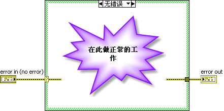
When the "Error In" data signifies an error, it implies that the preceding program encountered an issue, triggering the "Error" branch of the case structure. Since an error has already occurred, the subVI bypasses running additional functions, instead passing the error information onward. As such, the "Error" branch typically does not contain any operational code.

Conversely, if the "Error In" data does not indicate an error, it suggests that the previous program executed successfully. In this scenario, the case structure activates the "No Error" branch, containing all necessary code for the VI's (Virtual Instrument) operation.

This approach to error handling is a widely-used practice in LabVIEW. The intricacies of this mechanism will be more thoroughly explored in the Error Handling Mechanism section of this book.

Other Data Types

Case structures in programming can handle different data types, such as strings, integers, and Enum. Unlike Boolean data, which is limited to "True" or "False" and typically requires only two branches, these data types often necessitate multiple branches due to their wider range of possible values.

When expanding a case structure to include additional conditions, you can easily add new branches. Simply right-click on the case structure's border and select "Add Branch After" or "Add Branch Before" from the context menu. To reuse code from an existing branch in the new one, choose "Duplicate Branch". Afterward, you can set the specific conditions for each new branch.

It's worth noting that a single branch can respond to multiple conditions. These conditions are separated by commas. For instance, as shown in the image below, the third branch of the case structure is programmed to trigger under three distinct conditions - when the input is either 2, 4, or 6:

Furthermore, condition labels can denote a range of values. This is indicated by placing two dots between the minimum and maximum values of the range. For example, in the case structure from the above image, the fourth branch covers a range of values from 7 to 11. Thus, any input falling within this range will activate this particular branch. The fifth branch is set to handle all values greater than or equal to 12. When dealing with strings as conditions, ranges can also be defined, with the string values corresponding to their ASCII codes.

It's crucial to ensure that each branch condition is unique within the structure. If a condition is duplicated across different branches, LabVIEW will flag an error, preventing the VI (Virtual Instrument) from running. This requirement for unique conditions ensures clarity and accuracy in the execution of the case structure.

caution

LabVIEW exhibits some peculiar behaviors when handling case structures with conditions of different data types, particularly concerning how it interprets range conditions.

For instance, when using integer data types in a case structure, a condition like 1..3 encompasses values 1, 2, and 3, allowing any of these to match the branch. However, this logic slightly changes when dealing with string data types. If the condition is specified as '1'..'3' with string values, only '1' and '2' are included in the range, excluding '3'. This subtle difference in behavior can lead to unexpected outcomes in the program's execution. The two case structures illustrated below exemplify this discrepancy. While they appear very similar, differing only in the data type of their condition, they produce different results:

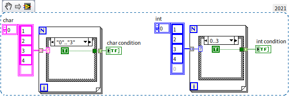
To correctly include the character '3' in a string condition range, the condition should be set as '1'..'4'. This is because, in string conditions, the upper limit of the range is exclusive. Therefore, to include all numeric characters from '0' to '9', the condition should be set as '0'..':' (since ':' is the ASCII character following '9'), or alternatively, as '0'..'9','9'. Similarly, to include the characters 'b', 'c', and 'd', you would set the condition as 'b'..'e'.

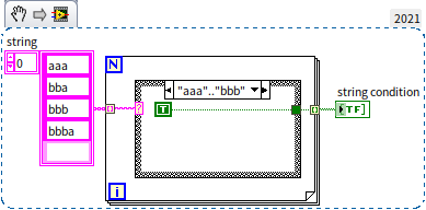
The distinct behavior of string conditions arises from the variable length of strings and the manner in which they are sorted. It is not feasible to directly define a string that precisely precedes a specific string. For instance, directly defining all strings beginning with the character 'a' is not straightforward. Therefore, we resort to using 'a'..'b' to denote all strings starting with 'a'.

Considering these nuances, readers are encouraged to think about what the outcome of the following program might be:

Default Branch

In some case structures, you might encounter branches labeled as "Default". This default branch comes into play when the input condition values don't match any of the specified branch conditions, leading the case structure to execute the code within the default branch. For Boolean data conditions, where only two branches (True and False) are typically needed, a default branch is usually unnecessary. However, with other data types, if the case structure's branches don't account for all potential condition values, LabVIEW will flag an error, preventing the VI from running. For instance, in the program shown below, the condition is an integer type, but the branches fail to handle values 0 and 1, causing an error:

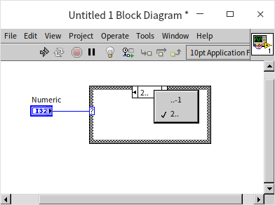
In such scenarios, you have a couple of options. You can designate one of the existing branches as the default by right-clicking it and choosing "Make This The Default Case" from the context menu. Alternatively, you could add branches for the missing conditions or modify the condition ranges of the existing branches to include 0 and 1:

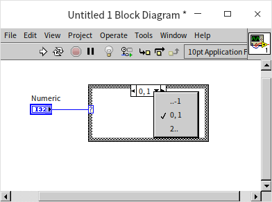
So, which approach is preferable? For beginners, opting for a default branch can be more straightforward and simplify the programming process. It's important to note that with Enum, where the number of values is finite, it's feasible to create a branch for each possible condition. However, in more complex projects, the focus shifts towards enhancing the program's stability, scalability, and maintainability. In such cases, a program designed to identify and address potential issues early on may be more advantageous than one that runs without immediate errors but has underlying issues.

From the standpoint of severity, a program that returns an error prompts the programmer to locate and fix the issue. However, a program that seems to run smoothly yet produces unexpected results for the client poses a more serious problem.

Another key factor is the cost associated with fixing errors. Often, the most time-consuming aspect of error resolution in programming isn't the modification itself, but the debugging process required to identify the error. For instance, a program that is almost error-free but has a 1% chance of randomly generating an erroneous result can be particularly challenging to debug due to the uncertainty surrounding the error's cause. On the other hand, a bug that causes a program to return an error code can be more easily addressed, as the error message provides valuable clues for quicker debugging. Ideally, a bug should be detectable at the compilation stage (i.e., preventing the VI from running), enabling the LabVIEW system to assist programmers in pinpointing the issue.

Consider the case of an Enum type condition. When initially designing a case structure, you may not foresee the need to add a new condition value in the future. This unforeseen condition might require specific handling within the case structure. If the VI is updated to include or rename an item in the Enum type without a default branch in the case structure, it will result in an error. In contrast, with a default branch, the VI won't trigger an error and will continue to operate.

From my personal experience, the approach varies based on the project scale. In smaller, simpler projects, the primary goal is often just to get the program running and producing results. However, in larger-scale projects, the focus shifts to enhancing program stability, scalability, and maintainability. In such scenarios, it's often more advantageous for a program with potential issues to fail early rather than later.

Optimizing Case Structures

A significant challenge with case structures is their limitation to displaying only one subdaigram at a time. This constraint can hinder code readability, as it may require flipping through various branches to understand the program fully. To counteract this, it's crucial to minimize the use of nested case structures and limit the number of branches during the design phase. Leveraging a branch selector that can handle multiple data types and allowing each branch to manage multiple conditions can greatly simplify your code.

Consider, for example, a scenario where you need to compare two integers, a and b. The goal is to display "a > b" if a > b, "a = b" if a = b, and "a < b" if a < b. While straightforward, strictly adhering to the program's logic might lead you to create nested case structures:

Nested structures can make reading the program more challenging due to the need to navigate between different sections. This can be improved by adjusting the program's logic to avoid nesting. For instance, using the difference between a and b as a basis for comparison can condense the logic into a single case structure:

An additional refinement in the above program is to extract the common "Single-Button Dialog" code from each branch and place it outside the case structure. This practice not only enhances readability but also improves the program's efficiency. Extracting and centralizing common code is a key strategy when working with case structures.

Here's another scenario: suppose you have two Boolean parameters, a and b, and you want to execute different actions based on their combined value. By forming a Boolean array from a and b and then converting it into a number, you can simplify the decision-making process. This approach allows you to use a single integer for logic determination, thereby avoiding nested structures:

Tunnel

Similar to loop structures, data flow in and out of case structures through tunnels. However, case structures have only one type of tunnel. When data flows into the case structure, the tunnel's input terminal is located on the structure's exterior, allowing connection to the output ends of other nodes. Inside the case structure, the tunnel's output terminal is accessible to each branch, enabling them to utilize the data received from the input terminal. In contrast, for data exiting the case structure through a tunnel, the output terminal of the tunnel is positioned outside the structure, while its input end is inside.

A key characteristic of case structures is that they execute the code from only one branch at any given time, with the specific branch to be executed during runtime remaining uncertain. This requires that data be provided to the input terminal of the output tunnel in every branch. Although this approach ensures that all branches are prepared to execute, it can become cumbersome, particularly because typically only one branch produces meaningful output for external code, while the others might only need to supply a default value. To streamline this process, a more efficient strategy is to configure the output tunnel with the "Use Default If Unwired" setting. When this option is activated, if any branch does not provide data to the input terminal of the output tunnel, the tunnel will automatically revert to the default value for that data type as its output. This approach simplifies the handling of branches that do not need to output specific data.

Deciding whether to enable the "Use Default If Unwired" setting on a tunnel parallels the earlier discussion about setting a default branch in case structures.

In numerous scenarios, a case structure's output tunnel is directly linked to an input tunnel. Unless specified otherwise by the program, the data exiting the structure should correspond to the data entering it. To efficiently link all branches that relate to these paired input and output tunnels, right-click on the output tunnel, choose "Connect Input Tunnels -> Create and Connect Unwired Branches", and then select the input tunnel. This action will seamlessly interconnect the input and output tunnels across all branches:

Avoid Placing Control Terminals Inside Case Structures

When developing a subVI that takes an integer "condition" and a floating-point array "input array" as input parameters, you might face a scenario where, if the "condition" value is 2, you need to increment each element in the "input array" and produce an output. Otherwise, no special processing is required. A common but flawed approach is to place controls within the case structure, as shown in the example below:

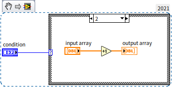
This approach presents two major issues:

1. Risk of Logical Errors: With the output control placed inside the branch for condition 2, if the program executes a different branch, the "output array" control will not receive any data. This leads to an indeterminate output value (which retains its last known value, but this value is unpredictable at runtime), potentially causing unexpected behaviors in the calling code.

2. Reduced Efficiency: Inserting input and output controls within the case structure can lead to performance degradation. This aspect is elaborated in the Memory Optimization section.

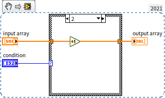
To circumvent these issues, it is advisable to place input and output controls outside of the case structure, as illustrated here:

tip

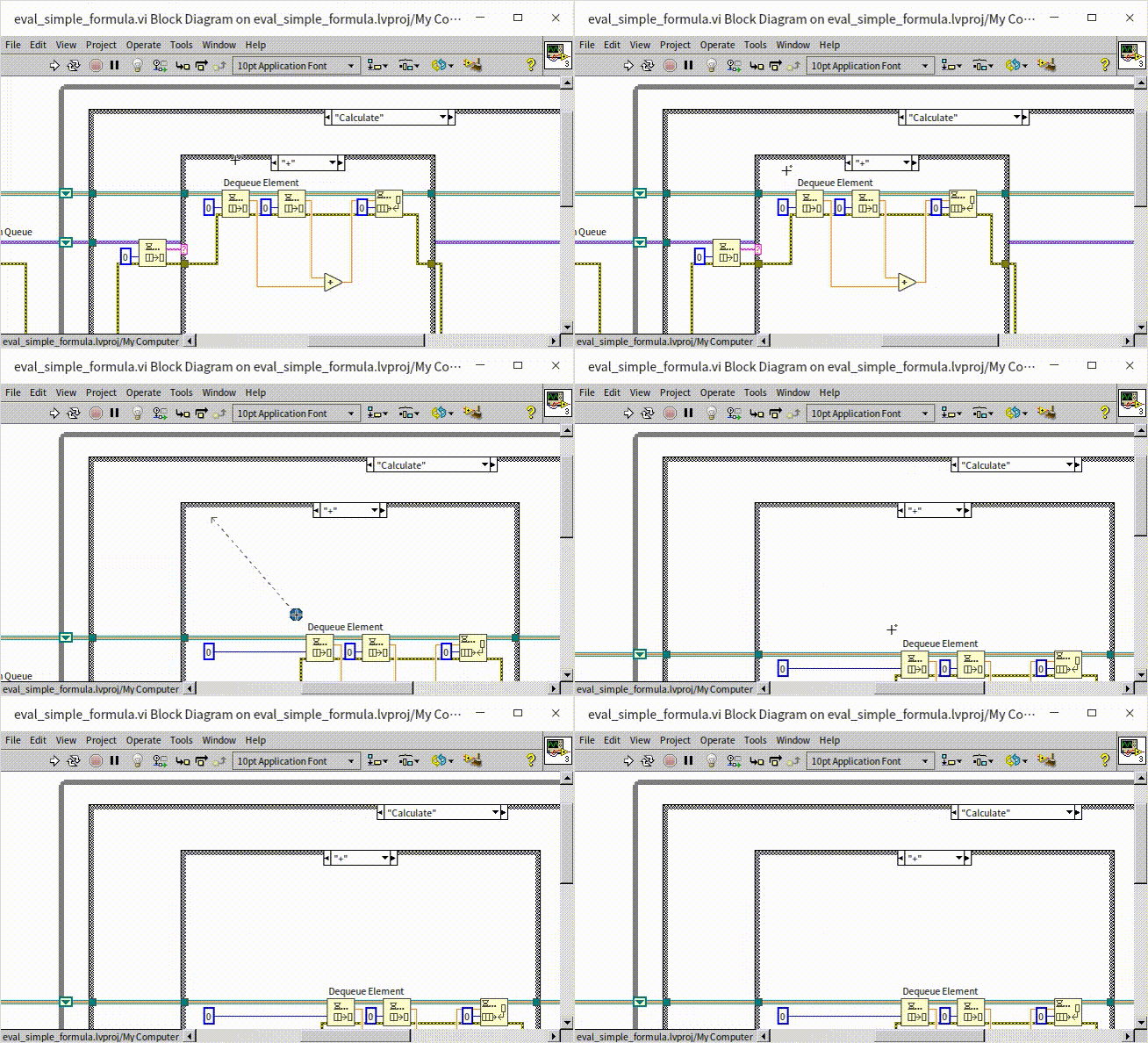
When you need to insert code into a densely populated area of your VI, a useful technique is to press and hold the Ctrl key, then click and drag the mouse to the desired insertion point. This action will shift adjacent code, creating space for the new code segment.

Selector Function

While case structures are a fundamental aspect of programming, they can sometimes suffer from readability issues. In certain scenarios, the Selector function offers a more readable alternative. You can find this function under "Programming -> Comparison -> Selector" in the function palette. The Selector function is equipped with three inputs. The second input specifically requires a Boolean data type, while the first and third inputs must share the same data type. Functionally, when the second input is "True" ,the Selector outputs the value from the first input. Conversely, if it's "False", the value from the third input is outputted. This resembles the x = c ? a : b; statement in C language.

In situations where a case structure's branch selector is either Boolean or can be converted to a Boolean type, and each branch's purpose is simply to choose between values, the Selector function can effectively replace the case structure. Take, for example, this segment of code we previously discussed:

Instead of the complex case structure, the same logic can be efficiently replicated using the Selector function, as depicted below:

The primary benefit of employing the Selector function lies in its ability to present all possible data choices directly on the block diagram. This greatly enhances the overall readability and clarity of the program.

sequence structure

Program Execution Order

LabVIEW's programming paradigm is driven by data flow, where the sequence of execution follows the data's path along the wires. Additionally, LabVIEW inherently supports multithreaded programming. This means that if two modules within a diagram are placed parallel to each other without any connecting wires, LabVIEW will automatically execute them concurrently in separate threads. Consider the following program:

In this example, data flows from the "error in" control, passes through "Sub VI A" and "Sub VI B", and then reaches the "error out" control. The execution sequence is dictated by this data flow: "Sub VI A" is processed first, followed by "Sub VI B".

Now, let's examine a case where two subVIs are executed in parallel:

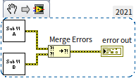
In this scenario, "Sub VI A" and "Sub VI B" are not interconnected by data wires, leading LabVIEW to treat them as independent entities and run them simultaneously. The "Merge Errors" function, located under "Programming -> Dialog & User Interface", is designed to amalgamate multiple error clusters into a single one. This function and its applications are discussed in detail in the Error Handling Mechanism section. Since "Merge Errors" receives input from both "Sub VI A" and "Sub VI B", the execution unfolds as follows: "Sub VI A" and "Sub VI B" commence concurrently, and after they have both completed, the "Merge Errors" function processes the aggregated data.

Implementing Sequence Structures

When you need to enforce a specific execution order for various functions or subVIs that are not connected by data wires, a sequence structure can be an effective solution. To add a flat sequence structure to your block diagram in LabVIEW, go to "Programming -> Structures -> Flat Sequence Structure" in the function palette.

Initially, when a sequence structure is placed on the block diagram, it appears as a dark gray box containing a single frame. You can add more frames by right-clicking on the structure and selecting the appropriate option from the context menu. Each frame within the sequence structure is capable of holding program code. During program execution, the sequence structure ensures that each frame is executed in a predefined order. Specifically, in flat sequence structures, the execution proceeds from left to right across the frames.

There are two ways to place a sequence structure on your block diagram: you can either add the structure first and then insert the desired code into it, or you can enclose existing code within a structure. The latter can be done by selecting the sequence structure tool from the function palette, dragging the mouse to form a rectangle around the code you wish to include, and then releasing the mouse button. This action creates a structure that encompasses the selected code.

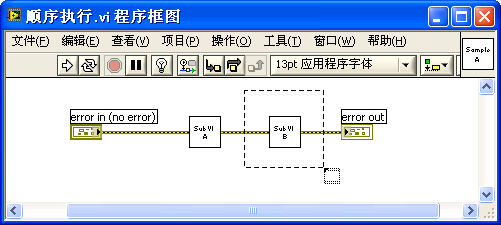
Here's an example of a properly placed sequence structure:

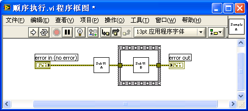
There are two types of sequence structures in LabVIEW: flat sequence structures and stacked sequence structures. Both types function similarly, with the primary distinction being how the frames are visually presented. In flat sequence structures, all frames are displayed side by side from left to right, allowing you to view the entire code sequence at a glance. Conversely, stacked sequence structures display only one frame at a time, with frame numbers above each frame indicating their order of execution.

Stacked Sequence Structure

Initially, LabVIEW only featured stacked sequence structures, and in later versions, these have been less emphasized in the function palette. This shift reflects the coding style LabVIEW now advocates. But let's start with an exploration of stacked sequence structures.

Suppose you need to develop a VI to measure the execution time of a code segment. The approach involves capturing the system time before and after the code runs. The difference between these two timestamps will indicate the code's execution duration.

For this task, since the time recording code and the test code are not interconnected by data wires but need to execute sequentially, a sequence structure is appropriate. Begin with a stacked sequence structure, which is divided into three frames: Frame 0 captures the current system time (pre-test code execution); Frame 1 houses the test code itself; Frame 2 records the system time once more (post-test code execution).

A challenge arises in this setup: Frame 2 requires the start time noted in Frame 0. Essentially, the time data generated in Frame 0 must be transferred to Frame 2. Direct wire connections between these two frames are not feasible since they are separate entities within the structure. To resolve this, the use of a "sequence local variable" is a suitable solution.

You can introduce a sequence local variable by right-clicking on the sequence structure's border and selecting the option to add one. This variable appears as a pale yellow rectangle, initially unconnected to any input data. Connect the output from the "Time Counter" function in Frame 0 to this newly created sequence local variable. Once connected to an input data wire, the sequence local variable will display an arrow inside the rectangle, color-coded to match the data wire. In the following frames, you can access the data stored in this sequence local variable as required, by connecting it with wires.

The arrow on a sequence local variable indicates the data flow direction: an arrow pointing toward the border signifies data entering the variable, while an arrow pointing away from the border indicates data exiting the variable. In sequence structures, a sequence local variable can be written in only one frame but can be read in any subsequent frames. In the frames preceding the one where data is written, the sequence local variable appears as a solid rectangle, signifying that it is neither readable nor writable at that point.

Sequence structures with stacked frames tend to suffer from readability issues. In the block diagram, only one frame is visible at a time, which makes it challenging to view the code in other frames and grasp the overall program logic.

Here is Frame 0 of our example program, employing the "Time Counter" function (located in the "Programming -> Time" palette) to record the current system time:

In Frame 1 of the stacked sequence structure, we have the test code. This code runs a loop until a randomly generated number matches a specified "comparison value". The function used here is "Random Number (0-1)" from the "Programming -> Numeric -> Random Number" palette.

Frame 2 of the structure reads the system time again and compares it with the time captured in Frame 0.

Data transfer into and out of a sequence structure is facilitated through tunnels, similar to those in loop and case structures. These tunnels are crucial for moving data in and out of the sequence structure. In such a structure, input tunnels allow data to be read by any frame, whereas output tunnels are designated to a single frame for writing data.

Identifying the origins or destinations of data within a sequence structure can be a complex task. For instance, in our example, data generated in Frame 1 exits the structure and feeds into the "Iteration Count" control. However, in Frames 0 and 2, the origins of this data are not visible. The source becomes apparent only when the structure is viewed in Frame 1. While navigating through a small three-frame structure like this may not be overly complicated, understanding the functionality in larger, multi-frame structures can be significantly more challenging.

The implementation of sequence local variables in stacked sequence structures tends to exacerbate readability challenges. Firstly, akin to tunnels, these variables necessitate a thorough examination of each frame to trace the data sources and the nodes receiving the data. Secondly, the fixed placement of a sequence local variable within each frame can lead to unconventional data flow directions, deviating from the standard left-to-right orientation.

In general practice, and particularly in text writing, the left-to-right flow is a familiar and expected direction. This expectation extends to programming in LabVIEW, where maintaining a left-to-right data flow direction is considered essential for readability and logical understanding. This principle is reflected in the design of most LabVIEW functions and subVIs, which typically position input parameters on the left and output parameters on the right.

However, when using sequence local variables, data flow often contravenes this principle. Take, for instance, Frame 0 in our program: the sequence local variable is placed to the left, and data from the "Time Counter" function flows towards this left-sided variable after capturing the current time. If the sequence local variable were positioned on the right, the data flow would indeed adhere to the left-to-right norm during the write operation. However, during the read operation in Frame 2, the data would then have to flow from right to left, which goes against this standard.

The origin of stacked sequence structures can be traced back to the limitations of early computer displays, which had relatively low resolutions and could not accommodate many functions and subVIs within a limited visible area. Stacked sequence structures were a solution to this constraint, allowing more code to be integrated into the same block diagram space. However, with the advent of modern large displays, the need for stacked sequence structures to condense code has diminished significantly.

Flat Sequence Structure

In the provided example, you can transform the stacked sequence structure into a flat sequence structure while retaining the same functionality. To do this, right-click on a frame of the sequence structure and select "Replace -> Replace with Flat Sequence Structure" from the menu. The flat sequence structure significantly improves readability:

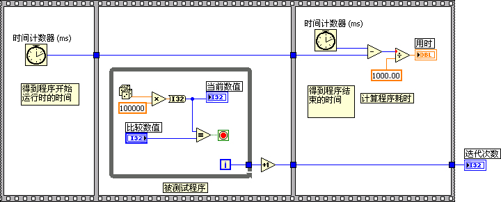
A key advantage of the flat sequence structure is its ability to display all frames simultaneously on the block diagram. This visibility eliminates the need for sequence local variables and allows users to easily comprehend the overall structure of the program. In the example shown, the source of the "Iteration Count" data is immediately apparent.

In a flat sequence structure, the code within each frame is executed sequentially from left to right. This alignment ensures that the execution order of the entire program follows a left-to-right progression, mirroring a natural and intuitive flow.

Given their superior readability, flat sequence structures are generally the preferred choice when a sequence structure is necessary. However, it's important to acknowledge that stacked sequence structures have their own benefits. One notable advantage is the ease with which the execution order of the frames can be adjusted — you can simply choose "Set Frame to..." from the right-click context menu of a stacked sequence structure to reorder the frames.

The Intangible Over the Tangible

In Chinese martial arts novels, it's often said that the zenith of swordsmanship is fighting as though the sword is not there. This concept can be analogously applied to sequence structures in programming: the ultimate mastery of using sequence structures is not needing to use them at all.

Consider a straightforward program that involves setting up an instrument and subsequently reading data from it. Crucially, after the setup, a brief pause is necessary for the configuration to stabilize before data can be accurately read. This requires implementing a one-second delay between the instrument's setup and the data reading to prevent inaccurate results.

Here's an initial attempt at such a program:

This approach, however, is flawed. The delay isn't linked to the instrument read/write operations via data wires, leading LabVIEW to execute both segments simultaneously. As a result, despite a one-second delay in the overall runtime, the timing of the instrument's read/write operations remains unaffected, leading to potential data inaccuracies. The program sequentially executes the "Set Instrument" and "Read Instrument Data" subVIs, but without considering the necessary delay.

In this example, "Set Instrument.vi" and "Read Instrument Data.vi" are placeholder subVIs, as indicated. The "Instrument Name" constant symbolizes a specific instrument, with detailed discussions on instrument handling reserved for the Measurement Applications The line connecting the subVIs at the bottom represents an error data wire. The "Wait (ms)" function, used for implementing delays, is part of LabVIEW's standard suite, located in the "Programming -> Timing" palette.

To achieve precise timing, the initial version of the program can be enhanced by incorporating a sequence structure:

Yet, this setup can be optimized further. In essence, the critical task is to control the execution order of the "Wait" function, and it's not necessary to enclose the other code within the sequence structure. This refined approach yields a more streamlined and clear program:

A crucial aspect to note is that in this program, the control over the execution order is primarily achieved through data connections rather than the sequence structure itself. By reconfiguring how data wires are connected, you can effectively manage the data flow and, consequently, the order of execution. Given that data wires are a prevalent means for controlling execution order in LabVIEW, it's feasible to replace all sequence structures by employing appropriate wiring strategies.

However, there is still a notable issue in the program. Regardless of whether an error occurs during the execution of "Set Instrument", the program proceeds with the "Wait" function, delaying for 1 second before concluding. Ideally, if an error is encountered in "Set Instrument", the program should bypass the wait and terminate immediately.

To address this, the delay part of the program can be encapsulated into a subVI. The following diagram illustrates this subVI:

This subVI incorporates a case structure to initiate the delay only if the "error in" input indicates no error. If an error is present, it skips the delay.

Upon optimizing the entire program, the final version appears as below, demonstrating how error wires can significantly enhance the readability and flow of program execution:

Employing this method to eliminate all sequence structures is a key strategy to make the code more efficient and uncluttered. A practical solution is to convert the contents of each frame of the sequence structure into a subVI, ensuring each has error inputs and outputs. This allows them to be interconnected using error wires, resulting in a program that comprises a series of sequentially connected subVIs. This creates a simple and easily understandable structure.

It's important to note that when the original version of the program was written, LabVIEW did not automatically include VIs with error inputs and outputs. However, modern versions of LabVIEW come equipped with such subVIs, like the "Time Delay" Express VI and "High Resolution Polling Wait.vi":

Practice Exercise

1. Arithmetic Expression Evaluator VI

   Develop a VI that processes a single string input control. This string should represent a basic arithmetic expression composed of three elements:

   • The first element is an integer.
   • The second element is an arithmetic operator, which could be addition (+), subtraction (-), multiplication (*), or division (/).
   • The third element is another integer.

   Examples of valid inputs include "23-6" or "445*78". Your VI should be capable of evaluating this input expression and outputting the result. For instance, if the input is "45+7", then the VI should output 52.

   Key Points:

   • Ensure your VI includes a parsing mechanism to correctly identify the integers and the operator in the input string.
   • Implement the logic to perform the arithmetic operation as per the identified operator.
   • Handle potential errors, such as division by zero or invalid inputs.

2. Runtime Measurement Program

   Create a new program in LabVIEW to measure the runtime of the Arithmetic Expression Evaluator VI you developed in the first exercise. This program should execute the Evaluator VI and record the time taken to complete the operation.

   Steps to Follow:

   • Utilize timing functions in LabVIEW, such as "Tick Count (ms)" or "High Resolution Relative Seconds", to capture the start and end times around the execution of your Arithmetic Expression Evaluator VI.
   • Calculate the difference between the start and end times to determine the runtime.
   • Consider adding functionality to run the Evaluator VI multiple times or with different inputs to assess its performance under various conditions.

   Considerations:

   • Ensure accurate timing by minimizing additional processing within the timing capture.
   • Be aware of the resolution of the timing function you choose to use, as it impacts the precision of your runtime measurement.