Basic Algorithms and Data Structures

Nicklaus Wirth, a distinguished Turing Award laureate and the creator of the Pascal programming language, introduced a fundamental concept: Program = Algorithm + Data Structure. Data structures focus on finding the most suitable way to organize data for a specific issue, while algorithms aim to discover the most efficient methods and procedures for solving that issue. Combined, they encapsulate what a program fundamentally is. This simplification, though not exhaustive, essentially captures the core nature of programming. Not surprisingly, questions about algorithms and data structures are among the most frequent during programming job interviews.

At the heart of LabVIEW programming lie algorithms and data structures as well. However, due to LabVIEW's long-standing application in developing test programs, which typically involves a limited variety of algorithms and data structures, their significance hasn't been as emphasized. Nonetheless, the impact of algorithms and data structures on the efficiency of program execution is crucial, surpassing the differences between using LabVIEW or C language. Understanding some fundamental algorithms and data structures can greatly enhance the efficiency of your programs. While there are often complaints about LabVIEW's execution speed, in reality, most programs have substantial room for optimization.

As two foundational aspects of programming, both algorithms and data structures could each fill an entire semester's course. In this section, given the constraints of space, we will only touch upon some elementary algorithms and data structures.

Time Complexity

This section closely relates to program execution efficiency, introducing a crucial metric for evaluating an algorithm's efficiency: algorithm complexity. Algorithm complexity divides into time complexity and space complexity. Space complexity refers to the memory space required for executing the algorithm. Generally, time complexity is of greater concern because it measures the workload needed to run an algorithm, directly affecting the algorithm's execution speed. Time complexity is expressed as a function, indicating that a high time complexity results in a substantial increase in workload with only a slight increase in input data. In contrast, algorithms with low time complexity don't significantly increase workload, even with a large increase in input. Time complexity varies with the problem at hand: some problems can be solved efficiently, while others lack a low-complexity solution. Thus, comparing time complexities of various algorithms for the same problem is meaningful.

Time complexity is denoted by the uppercase letter O, with a lowercase letter, such as $n$, representing the amount of data the algorithm processes.

• If an algorithm's runtime remains constant regardless of the input data size $n$, it indicates the algorithm operates at a constant level, denoted as $O(1)$.
• If an algorithm's runtime has a linear relationship with the input data size, for instance, the runtime is $c*n$ where $c$ is a constant, then the algorithm's time complexity is linear, represented as $O(n)$.
• If an algorithm's runtime is proportional to the square of the input data volume, its time complexity is $O(n^2)$; similarly, if the runtime is proportional to the cube of the input data volume, the complexity is $O(n^3)$, and so forth.

These levels are known as polynomial-level time complexities. Algorithms within this complexity range are typically viable for solving practical problems. However, if an algorithm's time complexity exceeds this range, like factorial-level $O(n!)$, exponential-level $O(2^n)$, or higher, it becomes practically unsolvable for real-world scenarios. We've previously discussed a Fibonacci number algorithm with a time complexity of $O(2^n)$, where ordinary computers struggle to solve problems with input values less than 20. Naturally, even within polynomial levels, finding the algorithm with the lowest complexity for a given problem is preferable.

Determining Prime Numbers

In this section, we delve into the time complexity of prime factorization algorithms. Given a number $n$ that is known to be the product of two prime numbers (without knowing which primes), what is the time complexity of factorizing $n$?

To illustrate more clearly, let's use specific numbers: suppose the primes are 17 and 19, their multiplication results in $17 \times 19 = 323$. For computers, multiplying two larger numbers takes nearly the same time as multiplying smaller ones, considered to be constant time, hence the complexity of multiplication is $O(1)$. However, factorizing 323 is not as straightforward. We can only start testing with the smallest prime and continue one by one. For instance, checking whether 323 is divisible by 2, then by 3, continuing until 17, where we finally find the answer. In the worst case, if $n$ is the product of two identical primes, we would need to search up to $\sqrt{n}$ times. Assuming multiplication and division take approximately the same amount of effort (though in reality, division is much slower), the time complexity of factorizing $n$ is $O(\sqrt{n})$. Here's a program for decomposing the product of two primes:

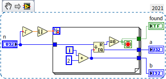
This program could be further optimized, for example, by ignoring factors that are clearly not prime (like even numbers). Despite these optimizations, its complexity remains at the $O(\sqrt{n})$ level, much higher than that of multiplying two primes. Indeed, $O(\sqrt{n})$ is considered very low among common algorithm complexities, yet it still struggles with particularly large inputs. If both primes are greater than $10^{10}$, factorizing their product with a conventional computer becomes impractically time-consuming. The significant difference in time complexity between an operation and its inverse has practical applications in computing, notably in encryption and decryption. The widely used RSA encryption algorithm exploits this feature, where multiplying primes is much quicker than decomposing a composite number into its prime factors. In simplified terms, the encryption and decryption process works as follows: Users A and B communicate over the internet, and all transmitted data (including the encryption algorithm and keys) can be intercepted by user C. To send a private message to A that C cannot understand, A first finds two large primes, then shares their product as the RSA algorithm's key with B. B uses this key to encrypt the message before sending it to A. Encryption requires only the composite number as the key, but decryption necessitates the original two primes, which A retains but C does not. If C wishes to decrypt, they must factorize the composite key, a relatively slow process. With sufficiently large primes chosen by A, C cannot determine the primes within a reasonable timeframe, effectively encrypting the information.

This encryption method is clever. However, it raises a question: Where does A find such large primes? A cannot simply select from a known list of primes because C might access the same list. If A generates a large random number, how can they ensure it's prime without factorizing it, which would require as much time as C would need? Although A has more preparation time, using a time-consuming algorithm is inconvenient. Fortunately, there are extremely efficient algorithms for determining if a number is prime, using properties of primes. For example, if $a$ is a small prime (like 2, 3, 5) and $p$ is a large number under consideration, $a^{p-1}-1$ is divisible by $p$ if $p$ is prime. This criterion can be used to develop the following program to check if a number is prime, with certain precautions: some composite numbers may occasionally satisfy the formula, so it's wise to test several values of $a$. For integers within the valid range of U64, testing with the five smallest primes (2, 3, 5, 7, 11) is sufficient. Additionally, direct computation of $a^{p-1}$ in LabVIEW is impractical for large $p$, as $a^{p-1}$ would result in an exceedingly large number beyond the range of U64. Since only the remainder of $a^{p-1}$ divided by $p$ matters, multiplication can be broken down into smaller calculations, retaining only the significant low-order part of the result to stay within U64's limits.

The Python code for this algorithm is as follows:

def montgomery(n, p, m):
    k = 1
    n %= m 
    while p != 1:  
        if 0 != (p & 1):
            k = (k * n) % m
        n= (n * n) % m
        p >>= 1
    return (n * k) % m

def is_prime(n):
    if n < 2:
        return False
    for a in [2, 3, 5, 7, 11]: 
        if 1 != montgomery(a, n-1, n):
            return False
    return True

The LabVIEW code for this algorithm is shown below:

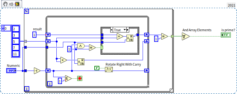
Using this program to sequentially test a range of integers quickly identifies some primes. For example, starting the search from 1,000,000,000, the program quickly finds a prime: 1,000,000,007.

Arrays

Efficiency of Basic Operations

Previously, in the section on Arrays and Loops, we introduced the fundamental operations of arrays in LabVIEW. This section will focus on the efficiency differences among various array operations, which largely depend on the method of array data storage in memory. Arrays store a sequence of data with the same type in contiguous memory spaces. Below is an illustration of how an integer array might be represented in memory:

Each element within the array is sequentially placed on a stretch of memory. This orderly arrangement greatly facilitates indexing to find or modify a specific array element. Given that each array element occupies a consistent amount of memory, the memory address of an element can be instantly calculated by: Element's memory address = Array's starting memory address + Index * Memory occupied by a single element. This indicates that the time complexity for accessing an array element is $O(1)$. However, this data organization method has its drawbacks, such as the relatively slow process of inserting or deleting an element within the array. Since each array element is sequentially placed, inserting or deleting an element in the middle necessitates shifting all subsequent elements either back or forward by one position. The worst-case scenario involves inserting an element at the array's start, requiring every element to shift back, essentially modifying all elements. The time complexity for inserting or deleting elements in an array is $O(n)$.

Consider a program that constructs an array of length 100,000, containing integers 0 to 99,999 in reverse order, from largest to smallest.

Given the integers are in reverse order, we can use the loop index as the data, inserting the index data at the array's beginning with each iteration to construct the required array. The program in the topmost sequence structure in the diagram below is implemented this way:

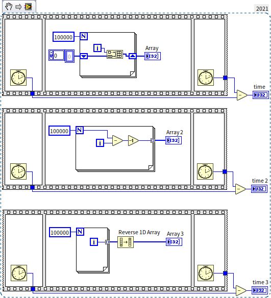
With the efficiency of each operation in mind, readers may have deduced that inserting data at an array's beginning is extremely slow. Each insertion carries a time complexity of $O(n)$, leading to a total complexity of $O(n^2)$ when inserting $n$ pieces of data. Thus, we should avoid array insertion in LabVIEW programs. The most natural and efficient way to construct arrays in LabVIEW is by using loop structures with all output tunnels. In the diagram, the two sequence structures below demonstrate better methods for constructing arrays. On my computer, the output values for time, time 2, and time 3 were 450, 1, and 2, respectively, showcasing the vast differences in efficiency.

info

Here's a thought for the readers: Inserting data at the array's start is evidently slow, but what about inserting at the end of the array? If the new element is the array's last, then moving other elements isn't necessary. Is that correct?

Multidimensional Arrays

Previously, we noted that LabVIEW does not support arrays of arrays due to the requirement for each array element to occupy a consistent amount of memory space. This consistency enables the rapid calculation of an element's memory location based on its index. However, arrays with varying numbers of elements have different lengths, complicating the indexing of a new array composed of these arrays. Instead, two-dimensional arrays can be employed to mimic arrays of arrays. Furthermore, arrays can be expanded to three dimensions or more. A two-dimensional array is essentially data arranged by rows and columns:

In memory, a two-dimensional array stores data row by row, with each row's data immediately followed by the next. Since each row has an identical number of elements, the memory address of any given element can still be instantly determined through its index. For example, in a two-dimensional array with $n$ rows and $m$ columns, to access the element at the $i^{th}$ row and $j^{th}$ column, the formula Element's memory address = Array's starting memory address + (m*i + j) * Memory occupied by a single element is used.

Nonetheless, LabVIEW permits arrays to contain elements whose lengths vary, such as in arrays of strings where each string's length differs. This is possible because when data types with variable lengths, like strings or clusters, are array elements, what is stored in the array are references to that data. The actual content of the string is stored in a different memory location. Regardless of the string's length, its reference is a 4-byte data, allowing the array to quickly find the element's memory address by its index. For more information on this topic, see the section on Flattening Data to Strings.

Sorting

Sorting a collection of data is a common task in programming, and LabVIEW offers built-in functions to sort elements within an array, ready for immediate use. In this section, we delve into the underpinnings of this sorting algorithm and discuss how to develop one's own sorting algorithms.

Let's think about how we typically sort items, such as organizing a bunch of apples by size from largest to smallest. Several methods come to mind:

• We often start by selecting the largest one from the pile, placing it in front of us; then we choose the next largest from the remaining apples to place it second, and so on. This sorting method is known as Selection Sort.
• Another preferred method involves: randomly picking an apple, comparing it with the ones we have, if the new apple is larger, it's placed in front, otherwise, it goes behind; then, we pick another apple and compare it with all the apples we have, positioning the new apple where it's smaller than the one before it but larger than the one after it. This sorting algorithm is called Insertion Sort.
• Bubble Sort is yet another similar algorithm: assuming we have an unsorted row of apples in front of us, we start by comparing the two apples on the far right, if the left one is larger, it stays put, if the right one is larger, they switch places; then we compare the second and third apples from the right, again switching them if the right one is larger; and continue this process. After one round, we ensure the largest apple is moved to the far left; repeating the operation ensures the second-largest apple moves next to it on the left; after $n$ rounds, $n$ apples are sorted.

These three algorithms are fairly simple and intuitive. Personally, I have a preference for Bubble Sort due to its relative simplicity and elegance in code representation. Below is the block diagram for a Bubble Sort program:

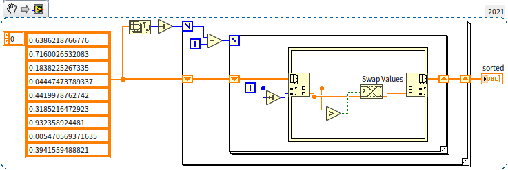
In these three sorting algorithms, placing each element in its correct position involves comparing or moving all other remaining elements. To sort $n$ pieces of data, $n$ rounds are needed, with each round performing an average of $n/2$ operations. Thus, the overall time complexity of these algorithms reaches a quadratic level, $O(n^2)$. If you test these algorithms with a large array, you'll find that they are significantly slower than LabVIEW's built-in sorting function. The reason for the slowdown is that sorting doesn't actually require comparing each element with all others. For instance, with three numbers $a$, $b$, and $c$, if it's already known that $a > b$ and $b > c$, then there's no need to compare $a$ and $c$. It's these unnecessary comparisons that decrease the efficiency of the aforementioned algorithms.

Some algorithms have optimized for this issue by eliminating redundant comparisons. Among them, Quick Sort is the most extensively used: continuing with the apple sorting example, we randomly select an apple as a pivot and compare all other apples with it. Those larger than the pivot are placed to its left; those smaller are placed to its right. This division creates three groups on the table: one in the middle, a group on the left, and a group on the right. It's guaranteed that any apple on the left is definitely larger than any apple on the right, thus eliminating the need for further comparisons between them. We then select a pivot from the smaller group of apples on the left, divide that group into even smaller groups using the same method, and apply the same process to the group on the right. Continuing this process until each small group contains only one apple completes the sorting.

This sorting algorithm removes all unnecessary comparisons, lowering its time complexity to $O(n\log_2 n)$. LabVIEW's built-in sorting function utilizes this type of algorithm.

Can it be even faster? For sorting through comparisons, with $n$ data items, you need at least $n*\log_2 n$ comparisons, so it's hard to speed up from there. But as mentioned earlier, the most efficient array operation is indexing. Could we sort by indexing rather than comparing? Indeed, there are such algorithms. For instance, to sort the integers 5, 4, 2, 8, 7, we could first create a counting array (hence the name Counting Sort), where the length of this auxiliary array must be greater than the largest number in the original array. For example, in our case, the largest number being 8 means we'd create a counting array of length 10. Next, we look at each number to be sorted, incrementing the corresponding element in the counting array by one. After counting is complete, a new array is constructed from the counting array to represent the sorted data. This approach is known as Counting Sort, and the diagram below illustrates its implementation:

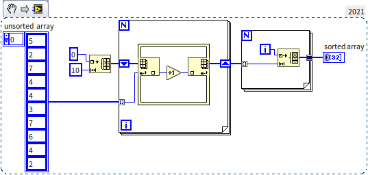
The time complexity of Counting Sort is $O(n)$, a level down from Quick Sort. From the program diagram, it's evident there are no nested loops, showing the computation count is linearly related to the input data length. Comparing the efficiency of Counting Sort with LabVIEW's built-in sorting:

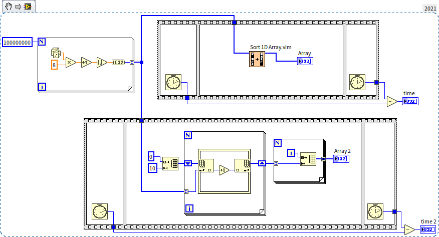
In the test program shown above, a random array of 100,000,000 numbers was generated and then passed to both LabVIEW's built-in sorting algorithm (upper sequence structure) and the Counting Sort algorithm (lower sequence structure). Running the program on my computer, the outputs for time and time 2 were 17156 and 93, respectively. This demonstrates that Counting Sort can significantly improve efficiency when used appropriately. So why doesn't LabVIEW's built-in sorting algorithm utilize Counting Sort?

As seen from the algorithm's description and implementation, basic Counting Sort is only suitable for sorting integer arrays within a small range of values. For other types of arrays, some processing can enable a $O(n)$ time complexity sorting algorithm:

• For integer arrays with a large range, they can be sorted digit by digit, handling just 0 to 9 at each step: first sorting by unit digit, then by tens, and so forth. This method is known as Radix Sorting.
• Original data can also be pre-processed to fit Counting Sort. For example, mapping all strings in a string array to a narrow integer range before sorting.

In essence, whether it's Radix Sorting or Counting Sort, their applicability is somewhat limited: programmers need to configure or even modify the algorithm for specific issues. A programming language's built-in function aims to be versatile, applicable across various data types. Sorting algorithms based on comparison have excellent versatility, allowing direct size comparisons for numbers, strings, or other common types without modification. Therefore, LabVIEW's built-in sorting function sticks with Quick Sort, making it adaptable for any user data. However, when we're writing our programs, if faced with sorting tasks requiring high efficiency, it's still worth considering implementing a custom $O(n)$ level sorting algorithm.

Search Algorithms

Another common operation with arrays is finding an element with a specific value. LabVIEW provides corresponding functions for this, offering two search functions: one for unsorted arrays and another for sorted arrays. For unsorted arrays, the only method is to compare each element sequentially until a match is found. In the worst case, this might mean comparing up to the last element to determine if the desired value is present, resulting in a time complexity of $O(n)$. However, for sorted arrays, a more efficient method exists. For instance, in an array sorted in descending order, we can compare the target value directly with the middle element of the array. If the target value is larger than this middle element, it indicates that the target must be on its left side, eliminating the need to search the right half of the array. Continuing this process on the left half until the target data is found. This algorithm, known as the Binary Search Algorithm, significantly reduces time complexity to $O(\log_2 n)$ by skipping most elements and only comparing a small subset.

The VI "Search Sorted 1D Array.vim" in LabVIEW, which is used for searching sorted arrays, is open-source. Readers can open its block diagram to learn how the binary search algorithm is implemented.

Similar to sorting, if searching can be based on indexing rather than numerical comparison, could it be quicker? Indeed, it can. For instance, if data in an array always corresponds to its index value, then to search for data 5, simply accessing the element at index 5 achieves this, reducing the search algorithm's complexity to $O(1)$. This data structure is a special combination of arrays with linked lists, known as a hash table or hashtable, which we'll discuss in more detail later.

Linked Lists

A linked list stores data in nodes, each comprising two parts: one for the data element and another for pointing to the next node in the sequence. This structure is depicted below:

In LabVIEW, implementing a generic linked list isn't straightforward; a more refined approach typically involves object-oriented programming. As such, this book will delve into how to implement a linked list after discussing object-oriented programming.

Linked lists offer relatively low efficiency for random data access but high efficiency for adding or deleting data, contrasting with array operations. The high efficiency in modifying linked lists stems from the fact that no other nodes need to be shifted around. To add data, simply insert a new node, making the previous node point to the new one, and then have the new node point to the subsequent node. Thus, without altering other data, new data is seamlessly integrated into the list. The deletion operation follows a similar logic, where you reconnect the preceding node directly to the node following the one being removed. Accessing data in a linked list by index has a time complexity of $O(n)$, while for arrays, it's $O(1)$. Conversely, adding or deleting data in a linked list has a time complexity of $O(1)$, compared to $O(n)$ for arrays.

This distinction suggests that arrays are more suited for storing data that requires frequent random access. For instance, signal data collected by hardware devices over a continuous period and stored in an array can be quickly accessed at any given moment. However, if data frequently needs to be added or removed, linked lists might be the preferable choice. For example, a program tasked with managing a list of work tasks, constantly adding new tasks and removing completed ones, could effectively utilize a linked list for this purpose.

It's worth noting that for small data volumes, such as a program managing information for a few dozen people in a department, the choice of data structure will not significantly impact performance. In such scenarios, the priority should be on development efficiency, favoring the use of readily available data structures or existing code.

Tree Structures

Tree Control in LabVIEW

In the linked list data structure, each node points only to the next node. If we modify this setup so that each node can point to several subsequent nodes, we create what's known as a tree data structure. This resembles an actual tree with many branches. While LabVIEW doesn't inherently provide a straightforward way to implement a generic tree data structure, it does feature a tree control. This control is specifically designed to display data in a hierarchical, tree-like format, such as for showcasing folders and files across multiple levels. The operation of the tree control closely mirrors how one would interact with a tree data structure. Thus, we can leverage the methods and properties of this control to delve into how tree data structures are manipulated. The appearance of the tree control is similar to that of a multi-column listbox, with the key distinction being in the leftmost column. While data in a multi-column listbox is displayed at a uniform level without any hierarchical distinction, the tree control differentiates levels through indentation:

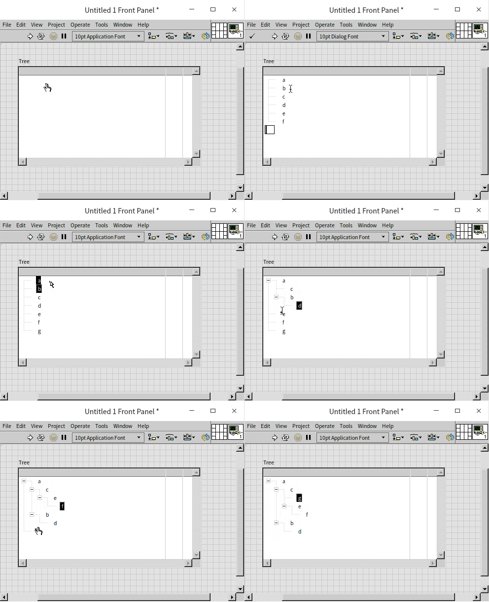
The illustration above demonstrates how items can be rearranged through drag-and-drop to establish hierarchical relationships directly within the interface.

Constructing a Sorted Binary Tree

The graphical representation of tree data structures closely matches the hierarchical layout presented by a tree control. Moving away from interface manipulation to programmatic construction, let's now build a tree through code. We will focus on constructing a Sorted Binary Tree.

A binary tree is defined as a tree in which each node has no more than two child nodes, meaning any branch can bifurcate into at most two branches. These child nodes are differentiated: we refer to them as the left and right child nodes. The left child node, along with all its descendants, forms what's called the node's left subtree; likewise, there's a right subtree.

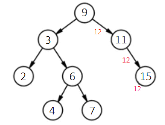
Sorting in a tree structure mandates that for any given node, its value must be greater than all values in its left subtree and less than all values in its right subtree. For instance, the tree shown below exemplifies a sorted binary tree:

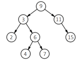
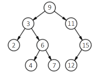
Firstly, each node in this tree has a maximum of two child nodes. Secondly, for any node, such as the topmost one (also referred to as the root node) with a value of 9, it is larger than any value in its left subtree and smaller than any value in its right subtree. When we wish to add new data, say 12, while ensuring the tree remains a sorted binary tree, we follow this procedure: Starting at the tree's root node, compare the new data, 12, with the root node's data, 9. Since 12 is larger, move to its right child node (if the new data were smaller, then move to the left child node). In the new child node, continue comparing the new data, 12, with the current node's data, 11. Because the new data is larger, proceed to 11’s right child node. In this node, since the new data, 12, is smaller than the node’s data, 15, it should enter the left child node. Given node 15 lacks a left child, a new node for the data 12 is created here, designating the new node as the left child of node 15. The process is illustrated as follows:

The tree post-insertion of the new node appears below:

Adhering to this logic, we can devise a program to sequentially construct a sorted binary tree using the data [9, 3, 2, 6, 4, 7, 11, 15, 12]. Given the tree control isn't expressly designed for tree data structures, for ease, we'll initially encapsulate its properties and methods into a sub VI for more straightforward manipulation of the data structure. The tree control poses two primary challenges for use as a data structure: firstly, whereas data structures typically utilize references to point to subsequent nodes, the tree control lacks element data references and instead employs tags to identify each data point. We must ensure each data point receives a unique tag. Here, we simplify matters by presuming no duplicates in the input data, thus allowing the data itself to serve as the tag. Another divergence lies in the tree control treating all a node's child nodes as equivalent without distinguishing left from right, whereas binary tree data structures necessitate distinguishing between left and right child nodes. To reconcile this, we prepend each data point's tag in the tree control with a prefix: "s" for the root node’s tag, "L" to denote all other left child nodes, and "R" for right child nodes. We encapsulate these adaptations in a sub VI "node_info.vi", showcased below in its block diagram:

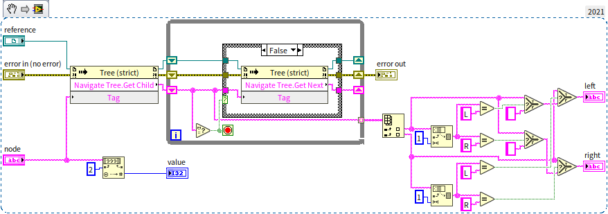
It inputs a node represented by a tag and outputs the data (value) stored in this node, along with its left child node (left) and right child node (right). By removing the prefix from the node's tag and converting it to a numerical data type, we get the data stored in the node. Next, the program calls the tree control's method for traversing nodes to get all the child nodes of the input node, then distinguishes between left and right child nodes based on the prefix of the child node being L or R.

With the aid of this sub VI, implementing the function to insert a node is quite straightforward. The program below is the block diagram for the "insert_node.vi":

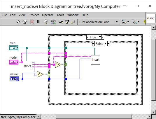
This is a recursive VI. The program first compares the size of the new data to the current data. If the new data is smaller, indicating that the new data should be placed in the current node's left subtree, the program checks if the current node has a left child node. If so, it recursively enters the left child node to continue comparing the new data with the left child node's data. If the current node lacks a left child node, then a new left child node is created with the new data:

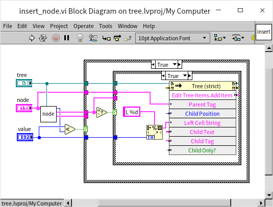
If the new data is greater than the current node's data, it should be inserted into the right subtree. The code for this is similar and hence not repeated. The main program for creating an entire tree is as follows:

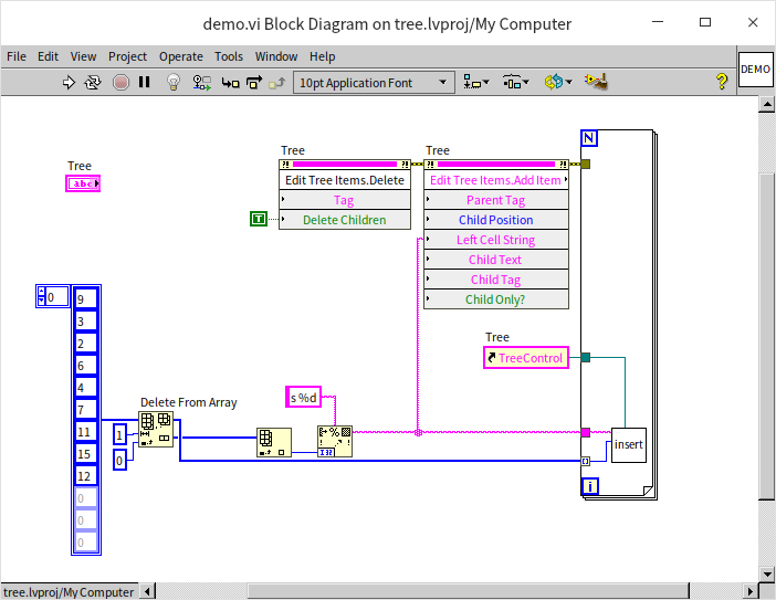
The main program first calls the tree control's "Delete" method to clear any pre-existing data in the control. It then uses the "Add Item" method to add the binary tree's root node, which has a distinct prefix, so it's added separately here. It then iteratively calls insert_node.vi to methodically add the remaining data to the tree. Running the above program, the tree control is displayed as follows:

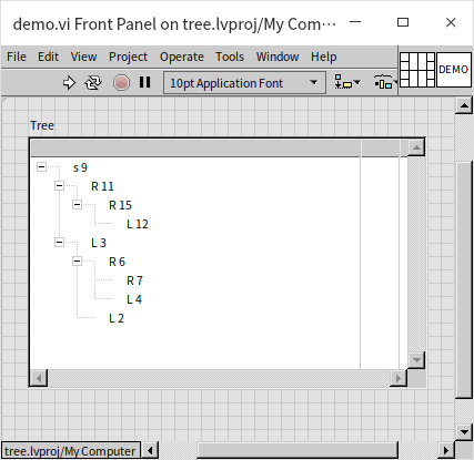
This tree's structure is consistent with the given illustrations. So, why create a sorted binary tree? Firstly, its efficiency in searching for data is exceptionally high, eliminating the need for comparing each piece of data individually. By comparing the data to be searched with the root node's data, it determines whether to search on the left or right, then continues this process in the subtree. This process is very similar to the binary search algorithm for sorted arrays mentioned earlier, which is why the sorted binary tree is also known as the Binary Search Tree. The search time complexity in a sorted binary tree is also $O(log_2 n)$. However, the efficiencies of inserting data differ significantly between the two. While inserting new data into a sorted array requires moving all elements behind the inserted element, resulting in a time complexity of $O(n)$; inserting a new node into a sorted binary tree does not necessitate moving any other nodes, with a time complexity of $O(1)$. However, it still needs to search for the placement of the new node, which has a time complexity of $O(log_2 n)$, making the overall process's time complexity $O(log_2 n)$. Overall, this efficiency is much higher than that of sorted arrays, thus sorted binary trees are often utilized in programs that require quick data queries, such as swiftly retrieving information about students in a school.

Tree Traversal

Tree traversal is another common algorithm for trees, involving visiting every node in a specified order. This process is also known as searching. The subtle difference between "traversal" and "searching" lies in the goals: traversal aims to visit every node without a specific target, while searching stops upon finding the target node, eliminating the need to visit others. In many scenarios, the terms traversal and searching are used interchangeably. When traversing a tree, one must decide between breadth-first (visiting all nodes at one level before moving to the next level) or depth-first traversal (exploring as far as possible along each branch before backtracking). Depth-first traversal further divides into: pre-order traversal (visiting the root node first, followed by the left child, then the right child), in-order traversal (left child first, then root, and finally right child), and post-order traversal (left child, right child, and root last). For sorted binary trees, in-order traversal results in a sequence sorted from smallest to largest. Below is the program for in-order traversal:

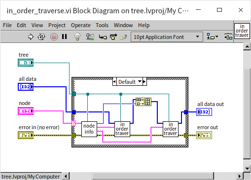
The program first checks if the input node is null; if so, it does nothing. Otherwise, it retrieves the node's data and its left and right children. In in-order traversal, the program recursively calls the traversal function for the left child node, inserts the data into the results, and then does the same for the right child node. Pre-order and post-order traversal simply rearrange these steps. In this demonstration, the traversal results are placed into an array. Although inserting data into an array is relatively inefficient, it's used here for easy demonstration on the front panel.

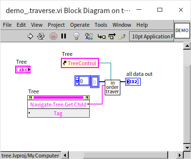
The main program for invoking in-order traversal is straightforward: get the root node and then call the traversal function:

Program execution result:

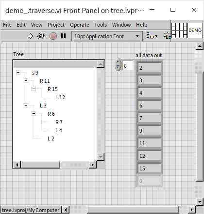
Tree traversal is an immensely useful algorithm. Many problems, including some that appear unrelated to trees, can be addressed using tree traversal, such as generating permutations of numbers, solving mazes, or tackling the 24-point problem: calculating 24 using addition, subtraction, multiplication, and division with four randomly chosen playing cards. Next, we'll explore a specific problem solved by employing tree traversal algorithms:

The Three Jug Puzzle

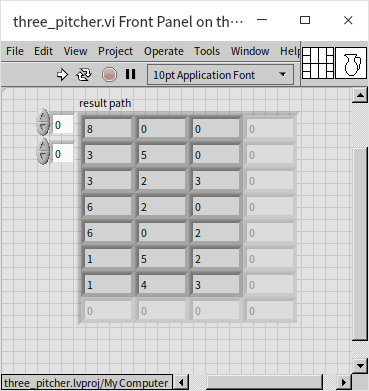
Suppose you have three jugs with capacities of 8 liters, 5 liters, and 3 liters, respectively. Initially, the 8-liter jug is full of water, and the other two are empty. How can you pour the water among the three jugs to exactly measure out 4 liters of water, using the fewest steps possible?

This puzzle might not seem related to trees at first glance. However, once you're familiar with tree traversal algorithms, solving it becomes straightforward. Even if you manage to measure exactly 4 liters by trial and error, you can't be sure you've found the most efficient solution without these algorithms.

The key is to construct a tree representing all possible states of the jugs and then traverse this tree to find the solution. Each state of the jugs (how much water each contains) is represented as a node in the tree. For instance, the initial state with 8, 0, and 0 liters is the root node, denoted as [8, 0, 0]. Its children represent all the states achievable by pouring water once. For example, from the root node, pouring water from the 8-liter to the 5-liter jug results in [3, 5, 0], and pouring into the 3-liter jug results in [5, 0, 3]. From [3, 5, 0], there are several possible actions leading to new states, and so forth. The diagram below illustrates a portion of this tree:

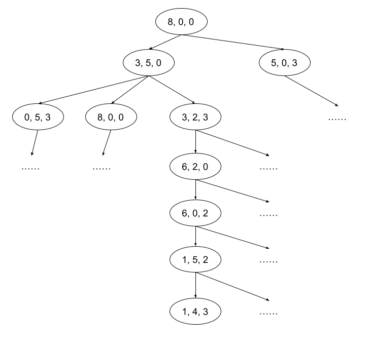
Within these nodes, some will contain the number 4 in their data. Finding a node closest to the root with 4 provides the puzzle's solution. The diagram above shows one potential solution, but it's not necessarily the most efficient. Verification through programming is required. We use a breadth-first search approach for this tree because we're looking for the solution with the fewest steps. We start with the root node and proceed to search all first-level child nodes, and so on.

In programming terms, we don't necessarily need to use the Tree Control or even construct a tree with nodes and references. Simply applying the tree traversal algorithm is sufficient. Below is how we approach the data in our program:

• A three-element integer array represents the state of the three jugs, with each element showing the water amount in each jug, e.g., [3, 2, 3]. The total water volume in the jugs is always 8 liters, with each jug's water level not exceeding its capacity.
• The capacities of the three jugs are represented by an integer array constant: [8, 5, 3].
• A cluster indicating the pouring direction has two integer elements: the first for the source jug and the second for the target jug, with values 0, 1, or 2, which must differ from each other.
• Six possible pouring methods exist for the three jugs, represented by an array constant.
• During pouring, if the target jug can accommodate all the water, then all the water from the source jug is poured in; otherwise, the target jug is filled to its capacity.
• Pouring operations can be ignored if the source jug is empty or the target jug is full.
• When the solution is found, the process, represented as a path from the root node to the solution node on the tree, is printed. This path records multiple nodes in a two-dimensional array, with each row representing a node.
• Each state in the program is passed around as a two-dimensional array representing its path. When traversing multiple states, the data becomes a three-dimensional array, with each path along the first dimension and the last data in each path representing the node under examination.

Having designed the data structures, we next develop a helper VI named "get_next_states.vi". This VI takes the current state of the jugs as input and outputs all possible next states:

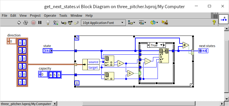
This program sequentially tries each of the six methods of transferring water between jugs. If a transfer is viable, it outputs the resulting new state. Essentially, this VI returns all potential child nodes of a given node within a tree-like structure.

The centerpiece VI for solving the three-jug puzzle utilizes the Breadth-First Search (BFS) algorithm, named "BFS.vi":

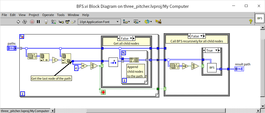
This VI, which is recursive, accepts a set of paths as input (each state is represented by a complete path), corresponding to all nodes at a specific level. Because it employs a breadth-first search approach, it first examines each input node for the presence of the number 4. If found, indicating a solution, the search concludes; otherwise, it invokes "get_next_states.vi" for each node to determine all next-level states, aggregating these into an array for recursive search through these new levels until a solution is identified.

The main program is straightforward, simply initiating the BFS VI with the root node:

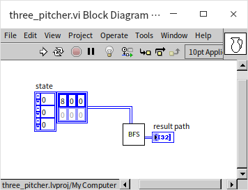
The output of the program, detailing each step to achieve the solution:

Although functional, this program exhibits a severe flaw due to many states repeating, such as water being poured back and forth between jugs A and B. These repetitions not only degrade efficiency but also risk trapping the program in an infinite loop if no solution is found. We will address these issues in subsequent discussions.

Notes on Using Tree Data Structures

While we demonstrated operations on tree data structures using the Tree Control for illustrative purposes, it's essential to remember that Tree Control is primarily designed for UI display and not as a data structure due to its inefficiency with large data volumes. In many applications, "trees" can be conceptually applied without the need to physically construct the tree with nodes and references. For instances requiring an actual tree structure, employing object-oriented programming methods, similar to those used for implementing a linked list, can create an efficient tree.

For a binary search tree to maintain its designed search efficiency, it must remain relatively balanced, where branch lengths are comparable. In extreme cases, a highly unbalanced tree can effectively become a linked list, drastically reducing search efficiency from the anticipated $O(log_2 n)$ to $O(n)$. While balancing a binary tree is possible, doing so constantly can be costly and potentially reduce overall efficiency. The Red-Black Tree, known for its self-balancing mechanism that minimizes unnecessary adjustments, is the industry's preferred binary search tree, offering an optimal balance of performance. LabVIEW internally uses Red-Black Trees for its collections and maps implementations.

Sets

Sets and maps, which I prefer to refer to as data containers, focus more on how to manipulate data rather than on the specifics of data storage. Calling them data structures is also appropriate, as the distinction between data containers and structures is often fluid. A set is designed to store and manage unique elements, and any data structure enabling this capability can be termed a set, whether the underlying storage mechanism involves arrays, linked lists, or trees. To ensure efficiency, LabVIEW implements sets using Red-Black Trees, enabling high-performance operations. Sets are particularly useful for ensuring data uniqueness; they can quickly determine if a piece of data is already present in the set and efficiently insert new data if not. Thanks to the Red-Black Tree implementation, both insertion into and querying of LabVIEW sets have a time complexity of $O(log_2 n)$. Below is a basic example of using a set:

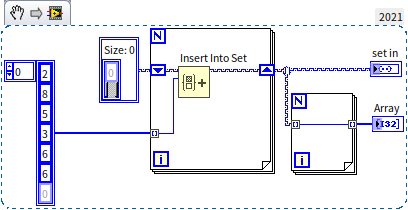
In this program, a sequence of integers in random order is inserted into a set, including the number 6 twice. However, since sets do not allow duplicates, the second instance of 6 is not added. The set resulting from running this program is sorted and devoid of duplicate entries:

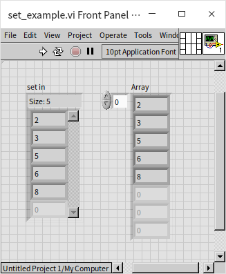
When set data is passed into a loop structure, it can be accessed using indexed tunnels just like with arrays. The retrieval order is based on their sorted order, not the order of insertion.

Given their properties, sets can often replace arrays in various applications, yielding superior performance. If a group of numbers requires sorting or must be unique, using a set instead of an array is advisable. Moreover, if an array doesn’t need to maintain its original sequence and often undergoes additions or deletions, considering a set as an alternative could be beneficial due to its higher efficiency in inserting and removing data.

In solving the three-jug puzzle described earlier, the program had a significant flaw: it encountered numerous duplicate nodes during tree traversal. We can utilize the unique properties of sets to address this issue effectively. The approach involves checking whether a newly created node is already present in a set; if it is, the node is ignored; if not, it is added to the set for further processing. The enhanced program is shown below:

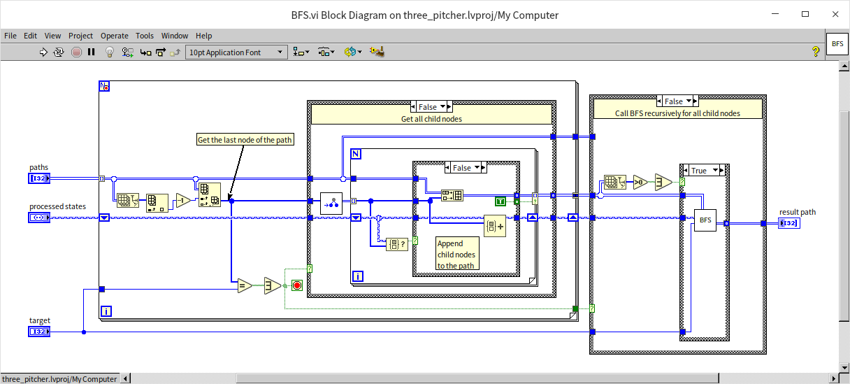
This updated breadth-first search algorithm closely resembles the previous version but includes a crucial enhancement: utilizing a set to verify whether a state has already occurred. By disregarding previously encountered states, the program not only becomes more efficient but also avoids potential infinite loops. When faced with an unattainable goal, such as achieving 9 liters, the program promptly returns an empty path, indicating that no solution exists.

Map

Sets use the data itself for comparison and search within the set. However, in many applications, the data users want to search by may not be the same as the data they're interested in retrieving. For example, in a program for querying exam scores, students are often looked up by their ID number, but the outcome sought is their exam score. For such applications, sets are inadequate. To address this, LabVIEW provides another very similar data container to sets called "maps". Maps and sets share the same underlying mechanism, but maps accompany each searchable piece of data with additional data. Thus, in a map, each node contains a pair of data: one termed as "key", used for comparisons and searches; and the other as "value", holding extra information related to the "key". A map that only contains "keys" without "values" essentially functions as a set. Taking the example of an exam score query program, student IDs can serve as keys, with their exam scores as values. If the need arises to view multiple scores, an array or cluster can be employed as the value to encapsulate multiple exam score data.

Beyond querying data, maps can also serve to optimize the efficiency of programs in certain scenarios. The most typical case is when a function that is time-consuming to execute might be called frequently within a short period using the same input parameters. In such instances, a map can be created for this function, with input parameters as the "key" and function outputs as the "value". This way, when the function is called, if the result for the given input parameters is already stored in the map, there's no need for recalculation; the cached result can be directly retrieved from the map. This book has utilized such an approach for optimization in the Recursive Algorithms section, more specifically in: Recursion with Caching.

Sets and maps were introduced as features in LabVIEW 2019. Prior to this, LabVIEW typically utilized variant data types to fulfill the functionalities of maps. If programs are seen using variant data types for data querying, it's likely because they were developed on an older version of LabVIEW.

Queue and Stack

Queues and stacks are two other extensively used data structures. Since this book has already thoroughly covered them in previous sections like Pass by Reference - Queue and State Machine, we will not reiterate those discussions here.

LabVIEW's queues are implemented using linked lists for data storage, hence the enqueueing and dequeueing operations have a time complexity of $O(1)$, which is highly efficient. In programs, if there is no requirement for random access within a collection of data and only the beginning or end of the data series needs to be accessed, opting for a queue over an array for data storage can significantly increase efficiency.